Downloading data and working with large data sets can be a challenge, especially when the data require aggregation. Overtime column names or file naming conventions may change, which lead to potential errors in the aggregation process. Other data sets involve so many files that it is impractical to forego automation.

In the biomedical sciences, there are many publically available Databases, Resources & APIs at the U.S. National Library of Medicine and U.S. Food & Drug Adminstration. For this blog, I’ve decided to share my approach to set up a small project using the FDA Adverse Event Reporting System (FAERS)(formerly AERS).

FAERS

The FAERS database contains adverse event and medication error reports that are submitted to the FDA, which are used to support post-marketing safety surveillance for drug and therapeutic biological products. Reports by healthcare professionals and consumers are voluntary, and details about the limitations and use of the data are found here.

Disclaimer*: My use of the FAERS here is solely to show one way to set up a database project, download and aggregate the data, and generate some simple graphs to illustrate some of the data of interest. I’m making no claims about the adverse health effects or drugs that are in the examples below. A full and formal analysis would require an in-depth consideration of the FAERS limitations, and a controlled statistical approach to the analysis. Further, the FAERS is designed to be used in a relational database system. Here, I’ve decided to forego this option, which may be more desirable depending on the goals of the project. Integration of R with SQL is fairly easy and is discussed elsewhere.

Project Folders

After a few years of R programming, I started to standardize the set up of all of my projects. Doing so enabled me to more easily transition projects to a High Performance Computing (HPC) node, and provided a clear way for others to implement the full project on their personal computers from scratch. Using the FAERS as an example, I set up projects in the following manner:

faers (parent project folder): Rmarkdown, and library and function scripts, .Rmd, .R, etc.
- zipfiles: downloaded raw data, .zip, .xml, etc.
- tables: individual raw data, .txt, .csv, etc.
- aggregate: aggregate raw data, .csv or .sql
- input: files and data required for analysis, .RData
- output: manuscript, reports, charts
- literature: publications, bibliography, .pdf, .bib, .csl, etc.

The settings I use in the following code chunk include: “```{r folders, echo=FALSE, eval=FALSE, error=FALSE, message=FALSE, warning=FALSE}”. Running this code chunk once will set up the project folders in a standardized manner. For the purposes of this blog to see the code chuck, I’m using ‘echo=TRUE’, which you would not normally show when knitting the document to a html, pdf, or doc for publication.

# do not run code chunk unless starting from scratch
dir.create("~/Documents/R/Databases/faers") # create a directory for the project
setwd("~/Documents/R/Databases/faers") # set up the working directory to the /faers folder
dir.create("zipfiles") # directory for zip files
dir.create("tables") # directory for unzipped files
dir.create("aggregate") # directory for agrgegate data
dir.create("input") # directory for input data for analysis, to include cleaned RData objects
dir.create("output") # directory for output of manuscripts, reports, graphs, etc.
dir.create("literature") # references, bibliography, csl

Libraries and Functions

For the next code chunk, I establish the main working directory, sub-directories, libraries and custom functions scripts.

In practice, I have one large libraries.R and custom functions.R scripts that I use with everything I do. This is probably a bad habit to load so many objects into the global environment, when most are not needed. Here, I’ve placed the essential libraries.R and functions.R source files in the main directory. These could be incorporated into the code chunk below, and avoid using source files all together. I’ve commented out this approach below each source file, which can also be found on my github page here.

setwd("~/Documents/R/Databases/faers") # set working directory

# Set working paths
maindir <- "~/Documents/R/Databases/faers/"
zipdir <- paste0(maindir, "zipfiles", "")
tabdir <- paste0(maindir, "tables", "")
aggdir <- paste0(maindir, "aggregate", "")
indir <- paste0(maindir, "input", "")
outdir <- paste0(maindir, "output", "")

# Load libraries and custom functions
source(paste0(maindir, "libraries.R", ""))

# # Packages
# cran_packages <-  c("ggplot2", "gridExtra", "data.table", "xml2", "rvest", "stringr", "readr")
# bioc_packages <- c("org.Hs.eg.db")
# 
# # Install if necessary:
# # install.packages(cran_packages)
# # source("https://bioconductor.org/biocLite.R")
# # biocLite(bioc_packages)
# 
# # Load packages into session
# sapply(c(cran_packages, bioc_packages), require, character.only = TRUE)

source(paste0(maindir, "functions.R", ""))

# ## CUSTOM FUNCTIONS ######################################
# ################################################################################
# 
# # FUNCTION TO TAKE LAST CHARACTER OF A STRING ##################################
# substrRight <- function(x, n) {
#   substr(x, nchar(x) - n + 1, nchar(x))
# }
# ################################################################################
# ################################################################################
# 
# 
# # FUNCTIONS TO NORMALIZE DATA ##################################################
# center_scale <- function(x) {
#   scale(x, scale = FALSE)
# }
# 
# normalizer <- function(x) {
#   (x-min(x))/(max(x)-min(x))
# }
# 
# center_apply <- function(x) {
#   apply(x, 2, function(y) y - mean(y))
# }
# 
# center_mean <- function(x) {
#   ones = rep(1, nrow(x))
#   x_mean = ones %*% t(colMeans(x))
#   x - x_mean
# }
# 
# center_sweep <- function(x, row.w = rep(1, nrow(x))/nrow(x)) {
#   get_average <- function(v) sum(v * row.w)/sum(row.w)
#   average <- apply(x, 2, get_average)
#   sweep(x, 2, average)
# }
# 
# # fastest way
# center_colmeans <- function(x) {
#   xcenter = colMeans(x)
#   x - rep(xcenter, rep.int(nrow(x), ncol(x)))
# }
# 
# center_operator <- function(x) {
#   n = nrow(x)
#   ones = rep(1, n)
#   H = diag(n) - (1/n) * (ones %*% t(ones))
#   H %*% x
# }
# ################################################################################
# ################################################################################
# 
# 
# # GGPLOT PUBLICATION THEME #####################################################
# theme_pub <- function (base_size = 12, base_family = "") {
# 
#   theme_grey(base_size = base_size, base_family = base_family) %+replace%
# 
#     theme(# Set text size
#       plot.title = element_text(size = 18),
#       axis.title.x = element_text(size = 16),
#       axis.title.y = element_text(size = 16,
#                                   angle = 90),
# 
#       axis.text.x = element_text(size = 14),
#       axis.text.y = element_text(size = 14,
#                                   angle = -45),
# 
#       strip.text.x = element_text(size = 15),
#       strip.text.y = element_text(size = 15,
#                                   angle = -90),
# 
#       # Legend text
#       legend.title = element_text(size = 15),
#       legend.text = element_text(size = 15),
# 
#       # Configure lines and axes
#       axis.ticks.x = element_line(colour = "black"),
#       axis.ticks.y = element_line(colour = "black"),
# 
#       # Plot background
#       panel.background = element_rect(fill = "white"),
#       panel.grid.major = element_line(colour = "grey83",
#                                       size = 0.2),
#       panel.grid.minor = element_line(colour = "grey88",
#                                       size = 0.5),
# 
#       # Facet labels
#       legend.key = element_rect(colour = "grey80"),
#       strip.background = element_rect(fill = "grey80",
#                                       colour = "grey50",
#                                       size = 0.2))
# }
################################################################################
################################################################################

Scraping ZIP Files

The full FAERS dataset can be found here. Again, since I only need to execute this code chunk once, I typically have ‘eval=FALSE’. Below, I download the ACIIS files. My experience with Structured Product Labels XML files leads me to believe that working with XML files is a littler trickier in general. In the future, I’ll add code to download and extract the data from the XML files.

# identify all the zip files you have downloaded previously, if any
current_sf <- list.files(path = zipdir, recursive = T, pattern = '*.zip' , full.names = T)
current_sf <- substrRight(current_sf, 13)

# identify the location and list of zip files to download
url <- "https://www.fda.gov/Drugs/GuidanceComplianceRegulatoryInformation/Surveillance/AdverseDrugEffects/ucm082193.htm"
pg <- read_html(url) # read page
links <- html_attr(html_nodes(pg, css = "a"), "href") # extract all nodes with href links
sublinks <- links[str_detect(links, '.zip')] # identify links to zip files
sublinks <- sublinks[!is.na(sublinks)] # remove any NAs
sublinks <- sublinks[str_detect(sublinks, current_sf)] # removes zip files that you already have downloaded previously

# loop to download ACIIS zip files and unzip
for (i in 1:length(sublinks)) {
download.file(url = paste0("https://www.fda.gov",sublinks[i], collapse = ''), dest = paste0(zipdir, "/", substrRight(sublinks[i], 13), collapse = ''), mode = "wget", method = "libcurl") # download zip files
unzip (paste0(zipdir, "/", substrRight(sublinks[i], 13), collapse = ''), exdir = paste0(zipdir, "/", i, collapse = '')) # unzip files
}

# list of all your ASCII files in the zip directory
sf  <- list.files(path = zipdir, recursive = T, pattern = '*.txt' , full.names = T)

Select ASCII Files of Interest

I’m primarily interested with indications, drugs, and reactions data files, but I provide the code for all 6 types of FAERS data sets. Depending on the year, the FDA labeled these with lower or upper case key words along with the year and quarter: ‘ther’, ‘rpsr’, ‘outc’, ‘indi’, ‘drug’, and ‘reac’. Below, I open all tables and convert them to .csv files. If you want to avoid keeping these separate files, it is perfectly reasonable to do so.

# list of key terms in ASCII file names to detect and aggregate
ft <- c("ther", "rpsr", "outc", "indi", "drug", "reac")
ft_cap <- c("THER", "RPSR", "OUTC", "INDI", "DRUG", "REAC")

# Loop to aggregate thrapy files, reaction files, drug files, etc.. across all years/quarters in FAERS and dump to aggregate_files folder
for (i in 1:length(ft)) {
  filt <- str_detect(sf, ft[i]) | str_detect(sf, ft_cap[i]) # FDA used different naming conventions, unfortunately
  hold <- sf[filt] # hold a subset, i.e. ther/THER files
  first_line <- c() # holder for the first line to read the header
  for (j in seq_along(hold)) {
    con <- file(hold[j],"r") 
    first_line[[j]] <- readLines(con, n = 1) # read first line of file
    close(con)
    dat <- read_table(hold[j]) # read in the table
    dt <- data.table(do.call(rbind, sapply(dat, function(x) str_split(x, "\\$")))) # split columns based on the $ delimiter
    cn <- sapply(first_line[[j]], function(x) str_split(x, "\\$")) # split column headers
    colnames(dt) <- unlist(cn)
    write.csv(dt, file = paste0(tabdir, "/", ft[i], "dt", j,".csv", ""), row.names = FALSE)
  }  
}

Aggregate Files

Next, I aggregate all the files with the key words in their file names. You might have noticed that I use data.table heavily, and in general avoid data frames in R. My goal is typically to shape the data I need for a project into a .RData object that is essentially a data.table, with all columns as characters, and no strings as factors.

# Loop to merge all aggregate data into single files
for (i in 1:length(ft)) {
  
  # re-establish ful file list based on the CSV files made 
  sf  <- list.files(path = tabdir, recursive = T, pattern = '*.csv' , full.names = T)
  
  hold <- sf[str_detect(sf, ft[i])] # subsetting the files
  
  dat <- read.csv(hold[1]) # starter data.table
  write.csv(dat, paste0(aggdir,"/agg", ft[i],".csv",""), row.names = FALSE)
  
  for (j in 2:length(hold)) {
    dat <- read.csv(hold[j])
    agg <- read.csv(paste0(aggdir,"/agg", ft[i],".csv",""))
    agg <- merge(agg, dat, all = TRUE)
    write.csv(agg, paste0(aggdir,"/agg", ft[i],".csv",""), row.names = FALSE)
  }
  
  # create the R objects
  agg <- data.table(agg)
  assign(ft[i], agg)
  write.csv(get(ft[i]), paste0("input/", ft[i],".RData",""), row.names = FALSE) 
}

# R objects created from the aggregate files
sf  <- list.files(path = indir, recursive = T, pattern = '*.RData' , full.names = T)

Example Analysis of Post-Traumatic Stress Disorder (PTSD) as an Adverse Drug Reaction (ADR)

For code chunks where you plan to have graphs and images, you need to set the options carefully. I use the following settings ‘```{r subset_data, echo = TRUE, eval = TRUE, message = FALSE, warning = FALSE, fig.height = 6, fig.width = 8, results = “asis”, digits = 3}’ for the next code chunk.

As a side note, on projects where there is heavy or lengthy computation, I often do not evaluate those code chunks every time that I wish to knit the html or pdf. I maintain the code chunk for reproducible research purposes, but rely on the very next code chunk to pull up a png image of the saved results.

If you were interested in another ADR, you can simply replace the “Post-traumatic stress disorder” with the “the ADR of interest.”

set.seed(100) # needed for reprodiucibility if using computations with random sampling

## Example of very simple analysis with these files
load(paste0(indir,"/drug.RData", collapse = ''))
load(paste0(indir,"/indi.RData", collapse = ''))
load(paste0(indir,"/reac.RData", collapse = ''))

# ADR of interest: replace with your interest and rerun to see results
adr_interest <- "Post-traumatic stress disorder"

# Example analysis with PTSD of interest
adr_primaryid <- reac$primaryid[reac$pt %in% adr_interest] # 1,215 elements with PTSD ADRs 

adr_reac <- reac[primaryid %in% adr_primaryid,] # 17,057 rows returned with PTSD primaryid

# create a table with the frequency of reactions in the PTSD ADR primaryid codes - i.e. co-ADRs
adr_coADRs <- data.table(table(adr_reac$pt)) # 2,362 coADRs
setnames(adr_coADRs, "V1", "reaction") # change column name
setorder(adr_coADRs, -N) # order based on most frequent ADR
adr_top10 <- adr_coADRs[2:11] # top co-ADRs (reaction): depression, anxiety, etc.. showing top 10.
pander(adr_top10) # can view as a table or..a graphic

reaction	N
Depression	400
Anxiety	355
Insomnia	190
Pain	185
Fatigue	168
Suicidal ideation	145
Drug ineffective	142
Headache	137
Nausea	119
Arthralgia	107

# top ten coADRs by frequency of total coADRs returned.
ggplot(adr_top10, aes(x = reorder(reaction, -N), y = N/sum(adr_coADRs$N))) + geom_bar(stat = "identity") + xlab("Adverse Drug Reaction") + ylab("Frequency") + ggtitle(paste0("Top 10 ", adr_interest, " co-ADRs", collapse = '')) + theme_pub() # I highly encourage setting up theme_pubs that you will use often, as it saves time.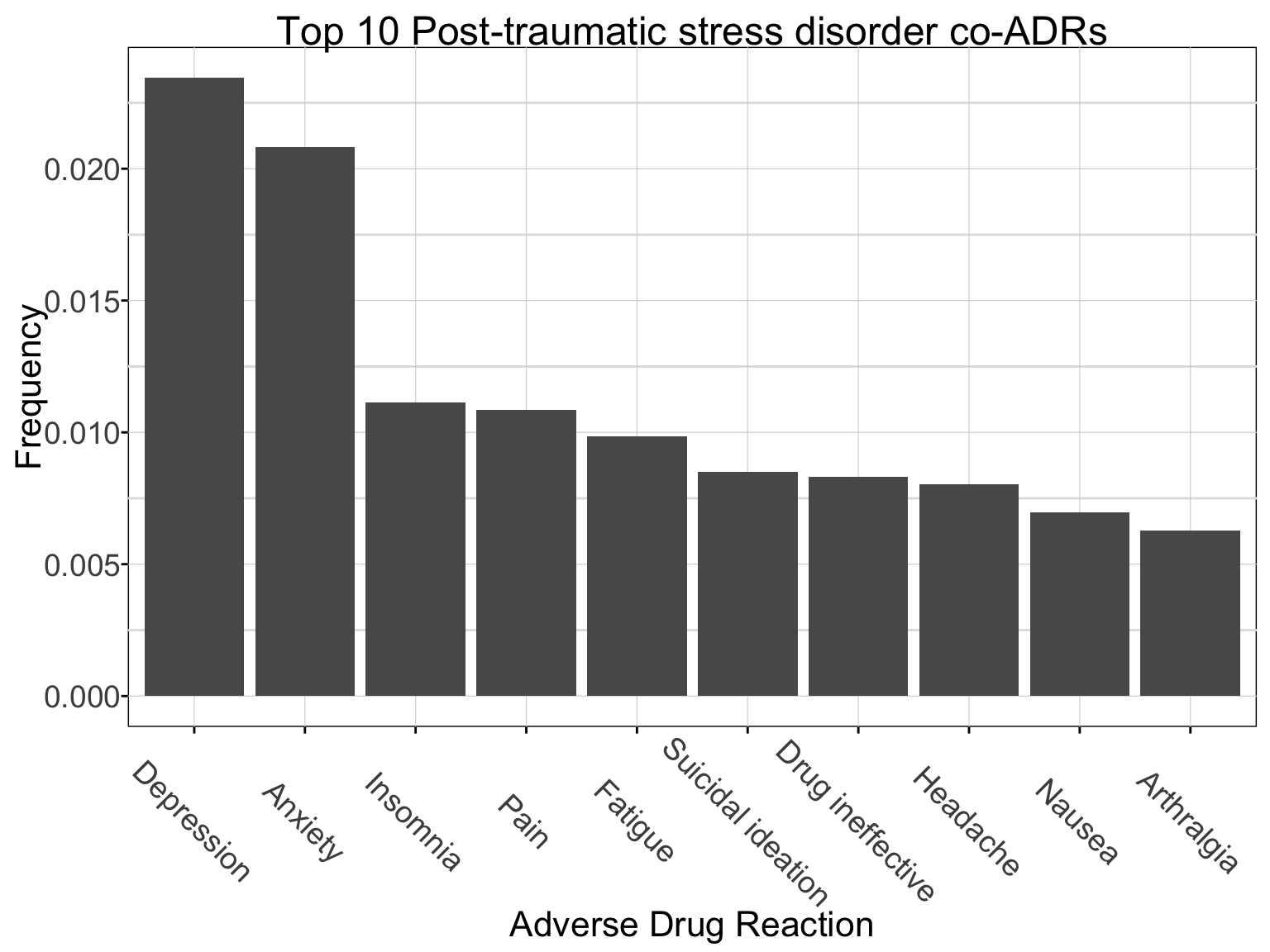

Suspected Drugs Releated to PTSD as an ADR

One column (‘role_cod’) in the ‘drug’ file indicates whether the drug is a primary, secondary, concomitant, or interacting suspect of the adverse drug reaction. Here, I’ve subset based on these factors and looked at the top 10 drugs by these categories.

codes <- c("PS", "SS", "C", "I") # suspected drug codes
titles <- c("Primary", "Secondary", "Concomitant", "Interacting")
adr_drugs_coADRs <- drug[primaryid %in% adr_reac$primaryid,] # subset the drug data file

# Loop to generate frequency table, filter top 10, and save graphics of results to an object 
for (i in 1:length(codes)){

adr_drugs <- adr_drugs_coADRs[role_cod == codes[i], .(drugname)] # subset based on suspect drug code
adr_drugs_N <- data.table(table(adr_drugs$drugname)) # use table function to see number of cases
setnames(adr_drugs_N, "V1", "drugname") # rename V1 column
setorder(adr_drugs_N, -N) # sort based on most frequent
adr_drugs_top10 <- adr_drugs_N[1:10] # select top 10 

p <- ggplot(adr_drugs_top10, aes(x = reorder(drugname, -N), y = N/sum(adr_drugs_N$N))) + geom_bar(stat = "identity") + xlab("Drugname") + ylab("Frequency") + ggtitle(paste0("Top 10 ", titles[i], " Suspect Drugs in ", adr_interest, collapse = '')) + theme_pub() # notice I devide the Number (N) by total cases in adr_drugs to obtain the frquency results that are displayed.

assign(codes[i], p) # assign the object a new name based on the iteration
}

# Uses extraGrid and cowplot to place all the figures in a single plot
plot_grid(PS, SS, C, I, labels = c("A", "B", "C", "D"), ncol = 1, nrow = 4, label_size = 32)

What’s Next

Now that we have identified the top drugs that are reported with the PTSD ADR, perhaps we could investigate further human genes that important to their mechanisms of action, or other interesting aspects of the drugs (just as an example). Over time, I’ll add in some code to show how to import human annotation data and extend the analysis a bit.

Until next time…

Jonathan D. Stallings #DataSolutions #DataScience #DataStories
jdstallings@DataInDeed.io

Example FAERS Project Setup