
Linear Regression
Linear regression is a very simple approach for supervised learning in order to find relationship between a single, continuous variable called dependent (or target) variable (i.e. numeric values, not categorical or groups) and one or more other variables (continuous or factor/groups) called independent variables. Thus, it can be used to predict a quantitative response. At least 5 cases per independent variable in the analysis is required. Many of the more sophisticated statistical learning approaches are in fact generalizations or extensions of linear regression.
Major Resources Used for This Post
- ‘Introductory Statistics with R’ by Peter Dalgaard
- ‘Discovering Statistics Using R’ by
- ‘An Introduction to Statistical Learning’ by Gereth James, et al.
- ‘Statistical Models: Theory and Practice’ by David Freedman
- ‘Statistical Models’ by A.C. Davison
- And several blogs that address this topic, see here.
Linear Regression
- Linear regression graphs a line over a set of data points that most closely fits the overall shape of the data in order to show the extent to which changes in a dependent variable (y axis) are attributed to changes in an independent variable (x axis).
- Example equation: \(Y = b_0 + b_1X_1 + b_2X_2 + b_3X_3 + ...... + b_kX_k\), where \(b_0\) is the intercept of the expected mean value of dependent variable (\(Y\)) when all independent variables (\(X\)) are equal to 0. \(b_1\) is the slope, which represents the amount by which the dependent variable (\(Y\)) changes if \(X_1\) was changed by one unit, while keeping other variables constant.
- Important term: Residual. The difference between observed values of the dependent variable and the value of the dependent variable predicted are residuals that from the regression line.
- Algorithm: Linear regression is based on least square estimation, which indicates regression coefficients (estimates) should be chosen in a manner to minimize the sum of the squared distances of each observed response to its fitted value (i.e. the least amount of information loss, see below.)
Example Uses in Business:
Evaluating Trends and Sales Estimates
- If a company’s sales have increased steadily every month for the past few years, conducting a linear analysis on the sales data with monthly sales on the y-axis and time on the x-axis would produce a line that that depicts the upward trend in sales.
- After creating the trend line, the company could use the slope of the line to forecast sales in future months.
Analyzing the Impact of Pricing Changes
- If a company changes the price on a certain product several times, it can record the quantity it sells for each price level and then perform a linear regression with quantity sold as the dependent variable and price as the explanatory variable.
- The result would be a line that depicts the extent to which consumers reduce their consumption of the product as prices increase, which could help guide future pricing decisions.
Assessing Risk
- A health insurance company might conduct a linear regression plotting number of claims per customer against age and discover that older customers tend to make more health insurance claims.
- The results of such an analysis might guide important business decisions made to account for risk.
Assumptions
- Linear Relationship: A linear relationship between the dependent and independent variable. Prior to conducting linear regression, you should explore the data by plotting the independent variable vs. dependent variables and run correlation between dependent variable and independent variables. There should be moderate and significant correlation score between them.
- When the error variance appears to be constant (homoscedasticity), only \(X\) needs be transformed to linearize the relationship.
- Transform independent variable to \(\log_{10} X\), \(f^{-1} X\), \(\sqrt X\), \(X^2\), \(\exp X\), \(1/X\), \(\exp (-X)\).
- When the error variance does not appear constant it may be necessary to transform \(Y\) or both \(X\) and \(Y\) (see below).
- Normaility of Residual: Linear regression requires residuals (the difference between an observed value of the dependent variable and the value of the dependent variable predicted from the regression line) should be normality distributed.
- Standardized Residuals is the residuals divided by the standard error of estimate (\(\sigma_{est} = \sqrt{\frac{\sum(Y-Y')^2}{N}}\)). It is a measure of accuracy of predictors.
- Studentized Residuals is the residuals divided by the residual standard error (\(RSE = \sqrt{\frac{\sum\hat e_i^2}{n-2}}\)) with that case deleted, where \(e\) is the residual error. If the absolute value of studentized residual is $ > 3$, the observation is considered as an outlier.
- Models with and without outliers have to be compared, and the smaller the the square root of the variance of the residuals, \(RMSE = \sqrt{\frac{\sum_{i-1}^n(X_{obs,i}-X_{model,i})^2}{n}}\), the better the model.
- It indicates the absolute fit of the model to the data–how close the observed data points are to the model’s predicted values.
- Whereas \(R^2 = (\frac{\sum_{i=1}^n(x_i - \overline x) \cdot (y_i - \overline y)}{\sqrt{\sum_{i=1}^n(x_i - \overline x)^2 \cdot \sum_{i=1}^n(y_i - \overline y)^2}})^2\) is a relative measure of fit, \(RMSE\) is an absolute measure of fit.
- Lower values of \(RMSE\) indicate better fit.
- Homoscedasticity: Linear regression assumes that residuals are approximately equal for all predicted dependent variable values.
- No Outlier Problem: By using the box plot method to identify any values that are \(1.5 \times IQR\) above the upper quartile (\(Q3\)) or below the lower quartile (\(Q1\)).
- Percentile capping based on distribution of a variable is used to deal with outliers by replacing extreme values with the largest/smallest non-extreme observation.
- Percentile capping based on distribution of a variable is used to deal with outliers by replacing extreme values with the largest/smallest non-extreme observation.
- Multicollinearity: It means there is a high correlation between independent variables. The linear regression model MUST NOT be faced with problem of multicollinearity.
- Independence of error terms - No Autocorrelation: It states that the errors associated with one observation are not correlated with the errors of any other observation. It is a problem when you use time series data. Suppose you have collected data from labors in eight different districts. It is likely that the labors within each district will tend to be more like one another that labors from different districts, that is, their errors are not independent.
Example Analysis
Downloading Data and Evaluating Linear Relationships
- An internal R data set called ‘mtcars’ was used to demonstrate the linear regression and resulting analysis.
- To examine the linear relationships we consider the following:
- Pearson correlation measures linear relationship of variables at interval scales, and is sensitive to outliers. A Pearson correlation of 1 indicates a perfect correlation, 0 indicates no linear relationship.
- Spearman’s correlation measures monotonic relationship, used for ordinal variables, and is less sensitive to outliers. Scores close to 0 indicate no monotonic relationship between variables.
- Hoeffding’s D correlation measures linear, monotonic and non-monotonic relationship. It has values between –0.5 to 1. The signs of Hoeffding coefficient has no interpretation.
- If a variable has a very low rank for Spearman (coefficient - close to 0) and a very high rank for Hoeffding indicates a non-monotonic relationship.
- If a variable has a very low rank for Pearson (coefficient - close to 0) and a very high rank for Hoeffding indicates a non-linear relationship.
- If a variable has poor rank on both the Spearman and Hoeffding correlation metrics, it means the relationship between the variables is random.
library(ggplot2)
library(car)
library(caret)
library(data.table)
library(kableExtra)

# Loading data
data(mtcars)
# Place data in a data.table with rownames
model <- data.table(model = rownames(mtcars))
model <- cbind(model, mtcars)

# Convert categorical variables to factor
model <- model[,"am" := as.factor(am)]
model <- model[,"cyl" := as.factor(cyl)]
model <- model[,"vs" := as.factor(vs)]
model <- model[,"gear" := as.factor(gear)]
model <- model[,"model" := as.factor(model)]

# Dropping dependent variable
model_dep <- subset(model, select = -c(mpg))

# Identifying numeric variables
numData <- model_dep[,sapply(model_dep, is.numeric), with = FALSE]
dt <- head(model)
data.table(dt) %>%
  mutate_if(is.numeric, format, digits = 2, nsmall = 0) %>%
  kable(.) %>%
kable_styling(bootstrap_options = "striped", full_width = F) | model | mpg | cyl | disp | hp | drat | wt | qsec | vs | am | gear | carb |
|---|---|---|---|---|---|---|---|---|---|---|---|
| Mazda RX4 | 21 | 6 | 160 | 110 | 3.9 | 2.6 | 16 | 0 | 1 | 4 | 4 |
| Mazda RX4 Wag | 21 | 6 | 160 | 110 | 3.9 | 2.9 | 17 | 0 | 1 | 4 | 4 |
| Datsun 710 | 23 | 4 | 108 | 93 | 3.9 | 2.3 | 19 | 1 | 1 | 4 | 1 |
| Hornet 4 Drive | 21 | 6 | 258 | 110 | 3.1 | 3.2 | 19 | 1 | 0 | 3 | 1 |
| Hornet Sportabout | 19 | 8 | 360 | 175 | 3.1 | 3.4 | 17 | 0 | 0 | 3 | 2 |
| Valiant | 18 | 6 | 225 | 105 | 2.8 | 3.5 | 20 | 1 | 0 | 3 | 1 |
- First, lets visualize the relationships with ggplot2:
fit <- lm(mpg ~ disp, data = model) # test linear relationship of mpg and disp
r2 <- paste("R^2:", format(summary(fit)$adj.r.squared, digits = 4))

g <- ggplot(model, aes(x = disp, y = mpg)) + geom_point()
g <- g + geom_smooth(method = "lm", se = T)
g <- g + annotate("text", x = 400, y = 30, label = r2)
g 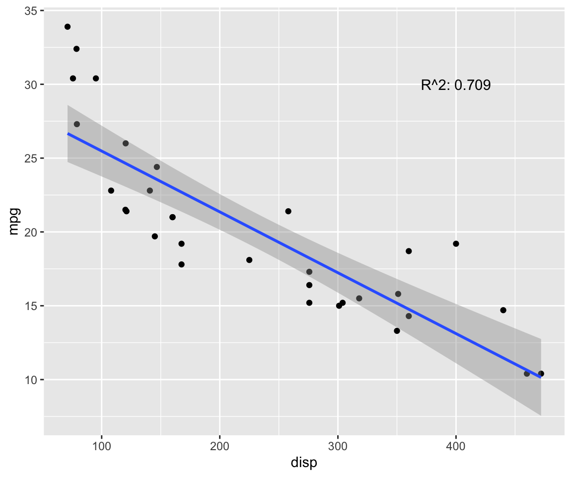
p.cor <- cor(model$disp, model$mpg, method = c("pearson"))
s.cor <- cor(model$disp, model$mpg, method = c("spearman"))
library(Hmisc)
h.cor <- hoeffd(model$disp, model$mpg)
cor <- data.frame("correlation scores" = c(p.cor, s.cor, h.cor$D[1,2]))
rownames(cor) <- c("pearson", "spearman", "hoeffd")
data.table(cor) %>%
  mutate_if(is.numeric, format, digits = 2, nsmall = 0) %>%
  kable(.) %>%
kable_styling(bootstrap_options = "striped", full_width = F) | correlation.scores |
|---|
| -0.85 |
| -0.91 |
| 0.47 |
fit <- lm(mpg ~ hp, data = model) # test linear relationship of mpg and hp
r2 <- paste("R^2:", format(summary(fit)$adj.r.squared, digits = 4))

g <- ggplot(model, aes(x = hp, y = mpg)) + geom_point()
g <- g + geom_smooth(method = "lm", se = T)
g <- g + annotate("text", x = 300, y = 30, label = r2)
g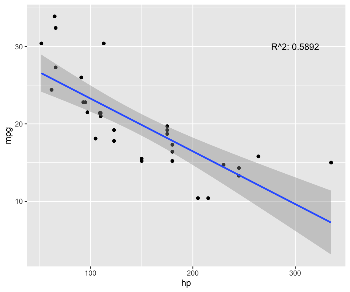
p.cor <- cor(model$hp, model$mpg, method = c("pearson"))
s.cor <- cor(model$hp, model$mpg, method = c("spearman"))
library(Hmisc)
h.cor <- hoeffd(model$hp, model$mpg)
cor <- data.frame("correlation scores" = c(p.cor, s.cor, h.cor$D[1,2]))
rownames(cor) <- c("pearson", "spearman", "hoeffd")
data.table(cor) %>%
  mutate_if(is.numeric, format, digits = 2, nsmall = 0) %>%
  kable(.) %>%
kable_styling(bootstrap_options = "striped", full_width = F) | correlation.scores |
|---|
| -0.78 |
| -0.89 |
| 0.48 |
fit <- lm(mpg ~ drat, data = model) # test linear relationship of mpg and drat
r2 <- paste("R^2:", format(summary(fit)$adj.r.squared, digits = 4))

g <- ggplot(model, aes(x = drat, y = mpg)) + geom_point()
g <- g + geom_smooth(method = "lm", se = T)
g <- g + annotate("text", x = 4.5, y = 12.5, label = r2)
g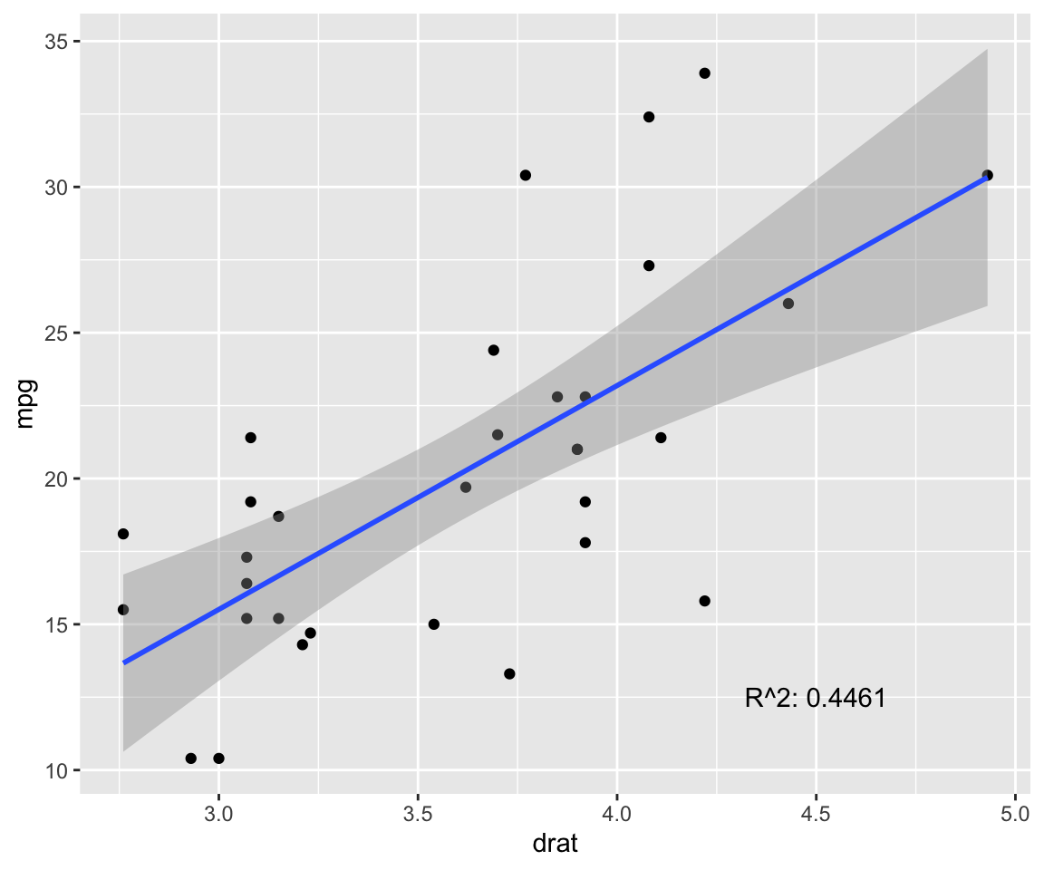
p.cor <- cor(model$drat, model$mpg, method = c("pearson"))
s.cor <- cor(model$drat, model$mpg, method = c("spearman"))
library(Hmisc)
h.cor <- hoeffd(model$drat, model$mpg)
cor <- data.frame("correlation scores" = c(p.cor, s.cor, h.cor$D[1,2]))
rownames(cor) <- c("pearson", "spearman", "hoeffd")
data.table(cor) %>%
  mutate_if(is.numeric, format, digits = 2, nsmall = 0) %>%
  kable(.) %>%
kable_styling(bootstrap_options = "striped", full_width = F) | correlation.scores |
|---|
| 0.68 |
| 0.65 |
| 0.13 |
fit <- lm(mpg ~ wt, data = model) # test linear relationship of mpg and wt
r2 <- paste("R^2:", format(summary(fit)$adj.r.squared, digits = 4))

g <- ggplot(model, aes(x = wt, y = mpg)) + geom_point()
g <- g + geom_smooth(method = "lm", se = T)
g <- g + annotate("text", x = 4.5, y = 30, label = r2)
g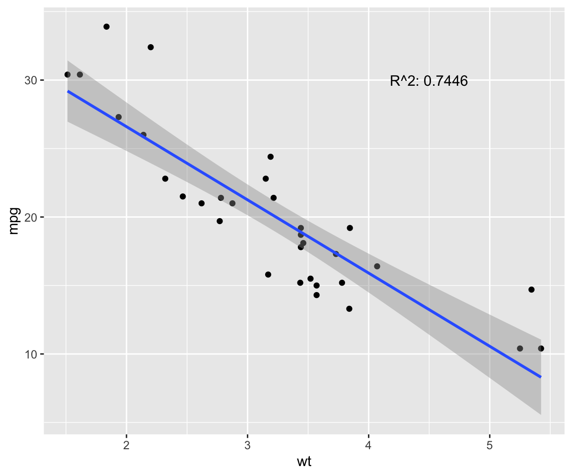
p.cor <- cor(model$wt, model$mpg, method = c("pearson"))
s.cor <- cor(model$wt, model$mpg, method = c("spearman"))
library(Hmisc)
h.cor <- hoeffd(model$wt, model$mpg)
cor <- data.frame("correlation scores" = c(p.cor, s.cor, h.cor$D[1,2]))
rownames(cor) <- c("pearson", "spearman", "hoeffd")
data.table(cor) %>%
  mutate_if(is.numeric, format, digits = 2, nsmall = 0) %>%
  kable(.) %>%
kable_styling(bootstrap_options = "striped", full_width = F) | correlation.scores |
|---|
| -0.87 |
| -0.89 |
| 0.41 |
fit <- lm(mpg ~ qsec, data = model) # test linear relationship of mpg and qsec
r2 <- paste("R^2:", format(summary(fit)$adj.r.squared, digits = 4))

g <- ggplot(model, aes(x = qsec, y = mpg)) + geom_point()
g <- g + geom_smooth(method = "lm", se = T)
g <- g + annotate("text", x = 21.5, y = 12.5, label = r2)
g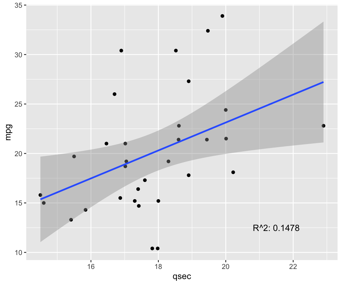
p.cor <- cor(model$qsec, model$mpg, method = c("pearson"))
s.cor <- cor(model$qsec, model$mpg, method = c("spearman"))
library(Hmisc)
h.cor <- hoeffd(model$qsec, model$mpg)
cor <- data.frame("correlation scores" = c(p.cor, s.cor, h.cor$D[1,2]))
rownames(cor) <- c("pearson", "spearman", "hoeffd")
data.table(cor) %>%
  mutate_if(is.numeric, format, digits = 2, nsmall = 0) %>%
  kable(.) %>%
kable_styling(bootstrap_options = "striped", full_width = F) | correlation.scores |
|---|
| 0.419 |
| 0.467 |
| 0.066 |
- If the assumption of linearity is violated, the linear regression model returns incorrect (i.e. biased) estimates, resulting in underestimated coefficients and \(R^2\) values.
Removing Highly Correlated Variables
- Removal of highly correlated variables reduces bias in the model.
- Using the correlation function, and plot has a heat map, you can quickly see which variables are highly correlated (i.e. blue boxes).
- Using the findCorrelation function, we can explicitly identify those variables that reach a certain threshold, such as a 0.6 cutoff.
- Using the correlation function, and plot has a heat map, you can quickly see which variables are highly correlated (i.e. blue boxes).
library(heatmap3)

# Calculating Correlation
descrCor <- cor(numData)
highlyCorrelated <- findCorrelation(descrCor, cutoff = 0.6)

# Identifying Variable Names of Highly Correlated Variables
highlyCorCol <- colnames(numData)[highlyCorrelated]

# Print correlated attributes
heatmap3(descrCor)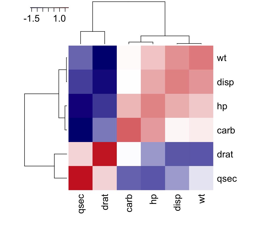
# Remove highly correlated variables and create a new dataset
dat3 <- model[, -which(colnames(model) %in% highlyCorCol), with = FALSE]- Here, I’ve specified the columns to use in the linear regression model. Alternatively, if you remove the ‘model’ columns earlier, you can just type mpg ~ . to conduct analysis on all the remaining columns in the data.table.
# Build Linear Regression Model
fit = lm(mpg ~ cyl + drat + qsec + vs + am + gear, data = dat3)

# Check Model Performance
summary(fit)
##
## Call:
## lm(formula = mpg ~ cyl + drat + qsec + vs + am + gear, data = dat3)
##
## Residuals:
## Min 1Q Median 3Q Max
## -6.3851 -1.5661 0.0514 1.5051 5.5417
##
## Coefficients:
## Estimate Std. Error t value Pr(>|t|)
## (Intercept) 11.9928 21.3463 0.562 0.5797
## cyl6 -4.3795 2.5905 -1.691 0.1044
## cyl8 -7.1791 4.0838 -1.758 0.0921 .
## drat 1.4201 2.4069 0.590 0.5609
## qsec 0.3208 0.8395 0.382 0.7059
## vs1 1.5841 2.5156 0.630 0.5351
## am1 4.6510 2.6219 1.774 0.0893 .
## gear4 -2.2463 2.8736 -0.782 0.4424
## gear5 -2.4115 3.0254 -0.797 0.4336
## ---
## Signif. codes: 0 '***' 0.001 '**' 0.01 '*' 0.05 '.' 0.1 ' ' 1
##
## Residual standard error: 3.287 on 23 degrees of freedom
## Multiple R-squared: 0.7793, Adjusted R-squared: 0.7026
## F-statistic: 10.15 on 8 and 23 DF, p-value: 5.862e-06- Additional information is extracted from the summary(fit) object with the $ operator, such as Coefficients (coeff), Rsquared values (r.squared), and adjusted Rsquared value (adj.r.square).
Measuring the Quality of the Statistical Models
- The Akaike information criteria (AIC) measures relative quality of statistical models given a set of data, which provides for model selection. AIC deals with trade-offs between goodness of fit of the model and model complexity.
- AIC calculates the Kullback-Leibler divergence, \(D_{KL}(f||g_1)\), to assess the loss of information from model to model. The model that minimizes information loss is selected.
- For more information see Akaike’s original 1973 manuscript.
- One limitation is small sample size, therefore, the estimate is only valid asymptotically. For smaller sample sizes, a correction (AICc) may be appropriate, see here.
- The Bayesian information criterion (BIC) or Schwarz criterion (SBC) is a criterion for model selection among a finite set of models; the model with the lowest BIC is preferred. For more information see Schwarz’s original 1978 manuscript.
AIC and BIC are both maximum likelihood estimators that introduce penalty terms for the number of parameters in the model in an effort to combat overfitting. They do so in ways that result in significantly different behavior. Lets look at one commonly presented version of the methods (which results from stipulating normally distributed errors and other well behaving assumptions):
\[AIC = 2k - 2ln(L)\], and \[BIC = ln(n)k - 2ln(L)\], where:
- \(k\) = model degrees of freedom, or free parameters to be estimated. In terms of linear regression, it is int he number of regressors including the intercept; \(\hat L\) = maximized value of the likelihood function of the model \(M\), i.e., \(\hat L = p(x|\hat \theta, M)\), where \(\hat \theta\) are the parameter values that maximize the likelihood function; \(n\) is the number of observations.
The best model in the group compared is the one that minimizes these scores, in both cases. Clearly, AIC does not depend directly on sample size. Moreover, generally speaking, AIC presents the danger that it might over fit, whereas BIC presents the danger that it might under fit, simply in virtue of how they penalize free parameters (\(2k\) in AIC; \(ln(n)k\) in BIC). Diachronically, as data is introduced and the scores are recalculated, at relatively low \(n\) (7 and less) BIC is more tolerant of free parameters than AIC, but less tolerant at higher \(n\) (as the natural log of \(n\) overcomes 2).
AIC Results:
# Stepwise Selection based on AIC
library(MASS)
step <- stepAIC(fit, direction = "both")
## Start: AIC=83.59
## mpg ~ cyl + drat + qsec + vs + am + gear
##
## Df Sum of Sq RSS AIC
## - gear 2 8.145 256.61 80.618
## - qsec 1 1.577 250.04 81.789
## - drat 1 3.761 252.23 82.067
## - vs 1 4.284 252.75 82.133
## <none> 248.47 83.586
## - cyl 2 35.897 284.36 83.905
## - am 1 33.994 282.46 85.690
##
## Step: AIC=80.62
## mpg ~ cyl + drat + qsec + vs + am
##
## Df Sum of Sq RSS AIC
## - drat 1 0.561 257.17 78.688
## - qsec 1 2.106 258.72 78.880
## - vs 1 3.217 259.83 79.017
## <none> 256.61 80.618
## - am 1 26.346 282.96 81.746
## - cyl 2 45.366 301.98 81.828
## + gear 2 8.145 248.47 83.586
##
## Step: AIC=78.69
## mpg ~ cyl + qsec + vs + am
##
## Df Sum of Sq RSS AIC
## - qsec 1 1.723 258.89 76.902
## - vs 1 3.427 260.60 77.112
## <none> 257.17 78.688
## - am 1 30.494 287.67 80.274
## + drat 1 0.561 256.61 80.618
## - cyl 2 58.713 315.88 81.269
## + gear 2 4.945 252.23 82.067
##
## Step: AIC=76.9
## mpg ~ cyl + vs + am
##
## Df Sum of Sq RSS AIC
## - vs 1 5.601 264.50 75.587
## <none> 258.90 76.902
## + qsec 1 1.723 257.17 78.688
## + drat 1 0.178 258.72 78.880
## - am 1 41.122 300.02 79.619
## + gear 2 6.300 252.60 80.114
## - cyl 2 94.591 353.49 82.867
##
## Step: AIC=75.59
## mpg ~ cyl + am
##
## Df Sum of Sq RSS AIC
## <none> 264.50 75.587
## + vs 1 5.60 258.90 76.902
## + qsec 1 3.90 260.60 77.112
## + drat 1 0.17 264.32 77.566
## - am 1 36.77 301.26 77.752
## + gear 2 6.74 257.76 78.761
## - cyl 2 456.40 720.90 103.672summary(step)##
## Call:
## lm(formula = mpg ~ cyl + am, data = dat3)
##
## Residuals:
## Min 1Q Median 3Q Max
## -5.9618 -1.4971 -0.2057 1.8907 6.5382
##
## Coefficients:
## Estimate Std. Error t value Pr(>|t|)
## (Intercept) 24.802 1.323 18.752 < 2e-16 ***
## cyl6 -6.156 1.536 -4.009 0.000411 ***
## cyl8 -10.068 1.452 -6.933 1.55e-07 ***
## am1 2.560 1.298 1.973 0.058457 .
## ---
## Signif. codes: 0 '***' 0.001 '**' 0.01 '*' 0.05 '.' 0.1 ' ' 1
##
## Residual standard error: 3.073 on 28 degrees of freedom
## Multiple R-squared: 0.7651, Adjusted R-squared: 0.7399
## F-statistic: 30.4 on 3 and 28 DF, p-value: 5.959e-09BIC Results:
# Stepwise Selection with BIC
n = dim(dat3)[1]
stepBIC = stepAIC(fit,k = log(n))
## Start: AIC=96.78
## mpg ~ cyl + drat + qsec + vs + am + gear
##
## Df Sum of Sq RSS AIC
## - gear 2 8.145 256.61 90.879
## - qsec 1 1.577 250.04 93.515
## - drat 1 3.761 252.23 93.793
## - vs 1 4.284 252.75 93.859
## - cyl 2 35.897 284.36 94.165
## <none> 248.47 96.778
## - am 1 33.994 282.46 97.416
##
## Step: AIC=90.88
## mpg ~ cyl + drat + qsec + vs + am
##
## Df Sum of Sq RSS AIC
## - drat 1 0.561 257.17 87.483
## - qsec 1 2.106 258.72 87.674
## - vs 1 3.217 259.83 87.812
## - cyl 2 45.366 301.98 89.156
## - am 1 26.346 282.96 90.540
## <none> 256.61 90.879
##
## Step: AIC=87.48
## mpg ~ cyl + qsec + vs + am
##
## Df Sum of Sq RSS AIC
## - qsec 1 1.723 258.89 84.231
## - vs 1 3.427 260.60 84.441
## - cyl 2 58.713 315.88 87.131
## <none> 257.17 87.483
## - am 1 30.494 287.67 87.603
##
## Step: AIC=84.23
## mpg ~ cyl + vs + am
##
## Df Sum of Sq RSS AIC
## - vs 1 5.601 264.50 81.450
## <none> 258.90 84.231
## - am 1 41.122 300.02 85.482
## - cyl 2 94.591 353.49 87.265
##
## Step: AIC=81.45
## mpg ~ cyl + am
##
## Df Sum of Sq RSS AIC
## <none> 264.50 81.450
## - am 1 36.77 301.26 82.149
## - cyl 2 456.40 720.90 106.604summary(stepBIC)##
## Call:
## lm(formula = mpg ~ cyl + am, data = dat3)
##
## Residuals:
## Min 1Q Median 3Q Max
## -5.9618 -1.4971 -0.2057 1.8907 6.5382
##
## Coefficients:
## Estimate Std. Error t value Pr(>|t|)
## (Intercept) 24.802 1.323 18.752 < 2e-16 ***
## cyl6 -6.156 1.536 -4.009 0.000411 ***
## cyl8 -10.068 1.452 -6.933 1.55e-07 ***
## am1 2.560 1.298 1.973 0.058457 .
## ---
## Signif. codes: 0 '***' 0.001 '**' 0.01 '*' 0.05 '.' 0.1 ' ' 1
##
## Residual standard error: 3.073 on 28 degrees of freedom
## Multiple R-squared: 0.7651, Adjusted R-squared: 0.7399
## F-statistic: 30.4 on 3 and 28 DF, p-value: 5.959e-09- As you can see, both AIC and BIC methods produce very similar results, and suggest the cyl6, cyl8, and am1 variables provide the least loss of information.
Standardize Coefficients
- Standardization or standardized coefficients (i.e. estimates) is important when the independent variables are of different units. In our case, mpg, cyl, disp, etc. all have different unit of measure. Therefore, if we were to rank their importance in the model, it would not be a fair comparison.
- The absolute value of standardized coefficients is used to rank independent variables, of which the maximum is most important.
library(standardize)
options(contrasts = c("contr.treatment", "contr.poly"))

dat3_std <- as.data.frame(dat3)
indx <- sapply(dat3_std, is.factor)
dat3_std[indx] <- lapply(dat3_std[indx], function(x) as.numeric(as.character(x)))
dat3_std[] <- lapply(dat3_std, function(x) if(is.numeric(x)){scale(x, center=TRUE, scale=TRUE)} else x)
fit_std = lm(mpg ~ cyl + drat + qsec + vs + am + gear, data = dat3_std)
stepAIC_std <- stepAIC(fit_std, direction = "both")
## Start: AIC=-34.37
## mpg ~ cyl + drat + qsec + vs + am + gear
##
## Df Sum of Sq RSS AIC
## - qsec 1 0.01200 7.0706 -36.313
## - vs 1 0.06181 7.1205 -36.088
## - drat 1 0.07302 7.1317 -36.038
## - gear 1 0.23021 7.2889 -35.340
## <none> 7.0587 -34.367
## - am 1 0.88543 7.9441 -32.586
## - cyl 1 1.17233 8.2310 -31.451
##
## Step: AIC=-36.31
## mpg ~ cyl + drat + vs + am + gear
##
## Df Sum of Sq RSS AIC
## - drat 1 0.06624 7.1369 -38.015
## - vs 1 0.08920 7.1598 -37.912
## - gear 1 0.29603 7.3667 -37.001
## <none> 7.0706 -36.313
## + qsec 1 0.01200 7.0587 -34.367
## - am 1 0.97832 8.0490 -34.166
## - cyl 1 1.98366 9.0543 -30.400
##
## Step: AIC=-38.01
## mpg ~ cyl + vs + am + gear
##
## Df Sum of Sq RSS AIC
## - vs 1 0.08706 7.2239 -39.627
## - gear 1 0.24182 7.3787 -38.948
## <none> 7.1369 -38.015
## + drat 1 0.06624 7.0706 -36.313
## + qsec 1 0.00522 7.1317 -36.038
## - am 1 1.18811 8.3250 -35.087
## - cyl 1 2.47199 9.6089 -30.498
##
## Step: AIC=-39.63
## mpg ~ cyl + am + gear
##
## Df Sum of Sq RSS AIC
## - gear 1 0.2466 7.4706 -40.552
## <none> 7.2239 -39.627
## + vs 1 0.0871 7.1369 -38.015
## + drat 1 0.0641 7.1598 -37.912
## + qsec 1 0.0261 7.1978 -37.743
## - am 1 1.1150 8.3389 -37.034
## - cyl 1 12.6210 19.8449 -9.289
##
## Step: AIC=-40.55
## mpg ~ cyl + am
##
## Df Sum of Sq RSS AIC
## <none> 7.4706 -40.552
## + gear 1 0.2466 7.2239 -39.627
## + qsec 1 0.1066 7.3640 -39.012
## + vs 1 0.0919 7.3787 -38.948
## + drat 1 0.0108 7.4597 -38.599
## - am 1 1.0178 8.4884 -38.465
## - cyl 1 12.3757 19.8462 -11.287n_std = dim(dat3_std)[1]
stepBIC_std = stepAIC(fit_std, k = log(n_std))## Start: AIC=-24.11
## mpg ~ cyl + drat + qsec + vs + am + gear
##
## Df Sum of Sq RSS AIC
## - qsec 1 0.01200 7.0706 -27.519
## - vs 1 0.06181 7.1205 -27.294
## - drat 1 0.07302 7.1317 -27.244
## - gear 1 0.23021 7.2889 -26.546
## <none> 7.0587 -24.107
## - am 1 0.88543 7.9441 -23.791
## - cyl 1 1.17233 8.2310 -22.656
##
## Step: AIC=-27.52
## mpg ~ cyl + drat + vs + am + gear
##
## Df Sum of Sq RSS AIC
## - drat 1 0.06624 7.1369 -30.686
## - vs 1 0.08920 7.1598 -30.583
## - gear 1 0.29603 7.3667 -29.672
## <none> 7.0706 -27.519
## - am 1 0.97832 8.0490 -26.837
## - cyl 1 1.98366 9.0543 -23.071
##
## Step: AIC=-30.69
## mpg ~ cyl + vs + am + gear
##
## Df Sum of Sq RSS AIC
## - vs 1 0.08706 7.2239 -33.764
## - gear 1 0.24182 7.3787 -33.085
## <none> 7.1369 -30.686
## - am 1 1.18811 8.3250 -29.224
## - cyl 1 2.47199 9.6089 -24.635
##
## Step: AIC=-33.76
## mpg ~ cyl + am + gear
##
## Df Sum of Sq RSS AIC
## - gear 1 0.2466 7.4706 -36.155
## <none> 7.2239 -33.764
## - am 1 1.1150 8.3389 -32.637
## - cyl 1 12.6210 19.8449 -4.892
##
## Step: AIC=-36.16
## mpg ~ cyl + am
##
## Df Sum of Sq RSS AIC
## <none> 7.4706 -36.155
## - am 1 1.0178 8.4884 -35.534
## - cyl 1 12.3757 19.8462 -8.356# R Function : Standardised coefficients
# stdz.coff <- function (regmodel)
# {
# b <- summary(regmodel)$coef[-1,1]
# sx <- sapply(regmodel$model[-1], sd)
# sy <- sapply(regmodel$model[1],sd)
# beta <- b * sx / sy
# return(beta)
# }
# std.Coeff = data.frame(Standardized.Coeff = stdz.coff(stepBIC_std))
# std.Coeff = cbind(Variable = row.names(std.Coeff), std.Coeff)
# row.names(std.Coeff) = NULL
# pander(std.Coeff)
summary(stepBIC_std)##
## Call:
## lm(formula = mpg ~ cyl + am, data = dat3_std)
##
## Residuals:
## Min 1Q Median 3Q Max
## -0.94337 -0.28492 -0.04409 0.31256 1.13065
##
## Coefficients:
## Estimate Std. Error t value Pr(>|t|)
## (Intercept) 1.126e-17 8.972e-02 0.000 1.0000
## cyl -7.411e-01 1.069e-01 -6.931 1.28e-07 ***
## am 2.125e-01 1.069e-01 1.988 0.0564 .
## ---
## Signif. codes: 0 '***' 0.001 '**' 0.01 '*' 0.05 '.' 0.1 ' ' 1
##
## Residual standard error: 0.5075 on 29 degrees of freedom
## Multiple R-squared: 0.759, Adjusted R-squared: 0.7424
## F-statistic: 45.67 on 2 and 29 DF, p-value: 1.094e-09- Thus, in our data, cyl6 is the most important variable.
Multicollinearity
- The variance inflation factors (VIF) function from the {car} package is used to calculate the variance-inflation and generalized variance-inflation factors for linear and generalized linear models.
- Variables with 1 degree of freedom (in our case, am) are calculated with the usual VIF, whereas, variables with more than one degree of freedom are calculated with generalized VIF.
- VIF for a single explanatory is obtained using the \(R^2\) value of the regression of that variable against all other explanatory variables: \(VIF_j = \frac {1}{1-R_j^2}\), where \(VIF\) for variable \(j\) is the reciprocal of the inverse of \(R^2\) from the regression. - As a rule of thumb, if \(VIF > 10\), then multicollinearity is high. For more info see this blog.
# Multicollinearity Test (Should be < 10)
# Check VIF of all the variables
data.table(vif(stepBIC)) %>%
  mutate_if(is.numeric, format, digits = 2, nsmall = 0) %>%
  kable(.) %>%
kable_styling(bootstrap_options = "striped", full_width = F) | GVIF | Df | GVIF^(1/(2*Df)) |
|---|---|---|
| 1.4 | 2 | 1.1 |
| 1.4 | 1 | 1.2 |
- In our data, the variables scored very low for multicollinearity.
Autocorrelation
- The Durbin-Watson statistic is a test for serial correlations between errors. It tests for the presence of autocorrelation (described as a relationship between values that is separated from each other by a given time lag) in the residuals (prediction errors) from a regression analysis.
- The test varies between 0 and 4, with the value of 2 indicated uncorrelated variables. Greater than 2 is a negative correlation between adjacent residuals, whereas a value less than 2 is a positive correlation. If the score is less than 1, there may be cause for alarm.
- If the \(e_t\) is the residual associated with the observation at time \(t\), then the test statistic is: \(d = \frac{\sum_{t=2}^T (e_t - e_{t-1})^2 }{\sum_{t=1}^T e_t^2}\), where \(T\) is the number of observations.
# Autocorrelation Test
durbinWatsonTest(stepBIC)
## lag Autocorrelation D-W Statistic p-value
## 1 0.1227506 1.619958 0.144
## Alternative hypothesis: rho != 0- In our data, the 1.6 D-W Statistic shows a small positive correlation, that is not statistically significant.
Normality of Residuals
- The Shapiro-Wilk test is a test of normality, which utilizes the null hypothesis principle to check whether a sample \(x_1,...x_n\) came from a normally distributed population: \(W = \frac{(\sum_{i=1}^n a_ix_{(i)})^2 }{\sum_{i=1}^n (x_i - \overline x)^2}\), where \(x(i)\) is the \(ith\) order statistic (smallest number in the sample) and \(\overline x = (x_1+...+x_n)/n\) is the sample mean and the \(a_i\) are given by \((a_1,...,a_n) = \frac{m^TV^{-1}}{(m^TV^{-1}V^{-1}m)^{1/2}}\), where \(m = (m_1,...m_n)^T\), and \(m_1,...,m_n\) are the expected values of the order statistics of independent and identically distributed random variables sampled from the standard normal distribution, and \(V\) is the covariance matrix of those order statistics.
# Normality Of Residuals (Should be > 0.05)
res = residuals(stepBIC, type = "pearson")
fit.standards <- rstandard(stepBIC)

qqnorm(fit.standards, ylab = "Standardized Residuals", xlab = "Normal Scores", main = "Q-Q Plot: Model (mpg ~.)")
qqline(fit.standards)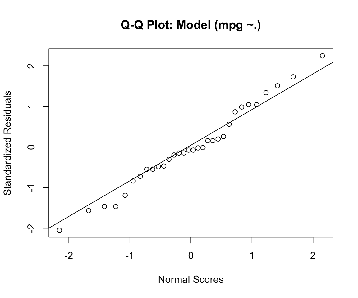
shapiro.test(res)##
## Shapiro-Wilk normality test
##
## data: res
## W = 0.98002, p-value = 0.8001- For our data, the Shapiro-Wilk test is not significant and we can not reject the null hypothesis that the data tested are from a normally distributed population.
Heteroscedasticity
- The ncvTest function tests whether the variance of the errors from a regression is dependent on the values of the independent variables.
- The test is often called Breusch-Pagan test, which returns a chisqTest object. The procedures involve some lengthy equations. Also, check out this blog for more information.
library(lmtest)
# Heteroscedasticity test (Should be > 0.05)
ncvTest(stepBIC)
## Non-constant Variance Score Test
## Variance formula: ~ fitted.values
## Chisquare = 3.40123, Df = 1, p = 0.065148# bptest(stepBIC) with the lmtest package the following matrix can be constructed
coeftest(stepBIC,vcov=hccm(stepBIC)) ##
## t test of coefficients:
##
## Estimate Std. Error t value Pr(>|t|)
## (Intercept) 24.8019 1.2554 19.7568 < 2.2e-16 ***
## cyl6 -6.1561 1.3282 -4.6349 7.522e-05 ***
## cyl8 -10.0676 1.4142 -7.1191 9.557e-08 ***
## am1 2.5600 1.1237 2.2782 0.03054 *
## ---
## Signif. codes: 0 '***' 0.001 '**' 0.01 '*' 0.05 '.' 0.1 ' ' 1# The actual model can be plotted to see all 4 charts at once.
par(mfrow = c(2,2)) # init 4 charts in 1 panel
plot(stepBIC)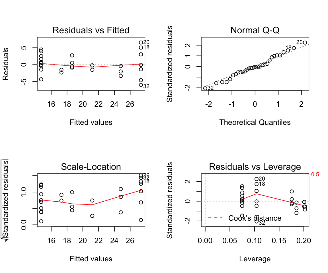
- For our data, the Non-constant variance score test has a p-value of 0.065, and therefore we can not reject the null hypothesis.
Outliers
- The outlierTest function reports the Bonferroni p-values for Studentized residuals in linear and generalized linear models, based on a t-test for linear models and normal-distribution test for generalized linear models.
- For a very in depth look at outliers see this blog. Further, this site helps to explain the interpretation of many these diagnostic plots.
# Outliers – Bonferonni test
outlierTest(stepBIC)
## No Studentized residuals with Bonferroni p < 0.05
## Largest |rstudent|:
## rstudent unadjusted p-value Bonferroni p
## 20 2.43792 0.021635 0.69232# Residuals
resid <- residuals(stepBIC)
leveragePlots(stepBIC)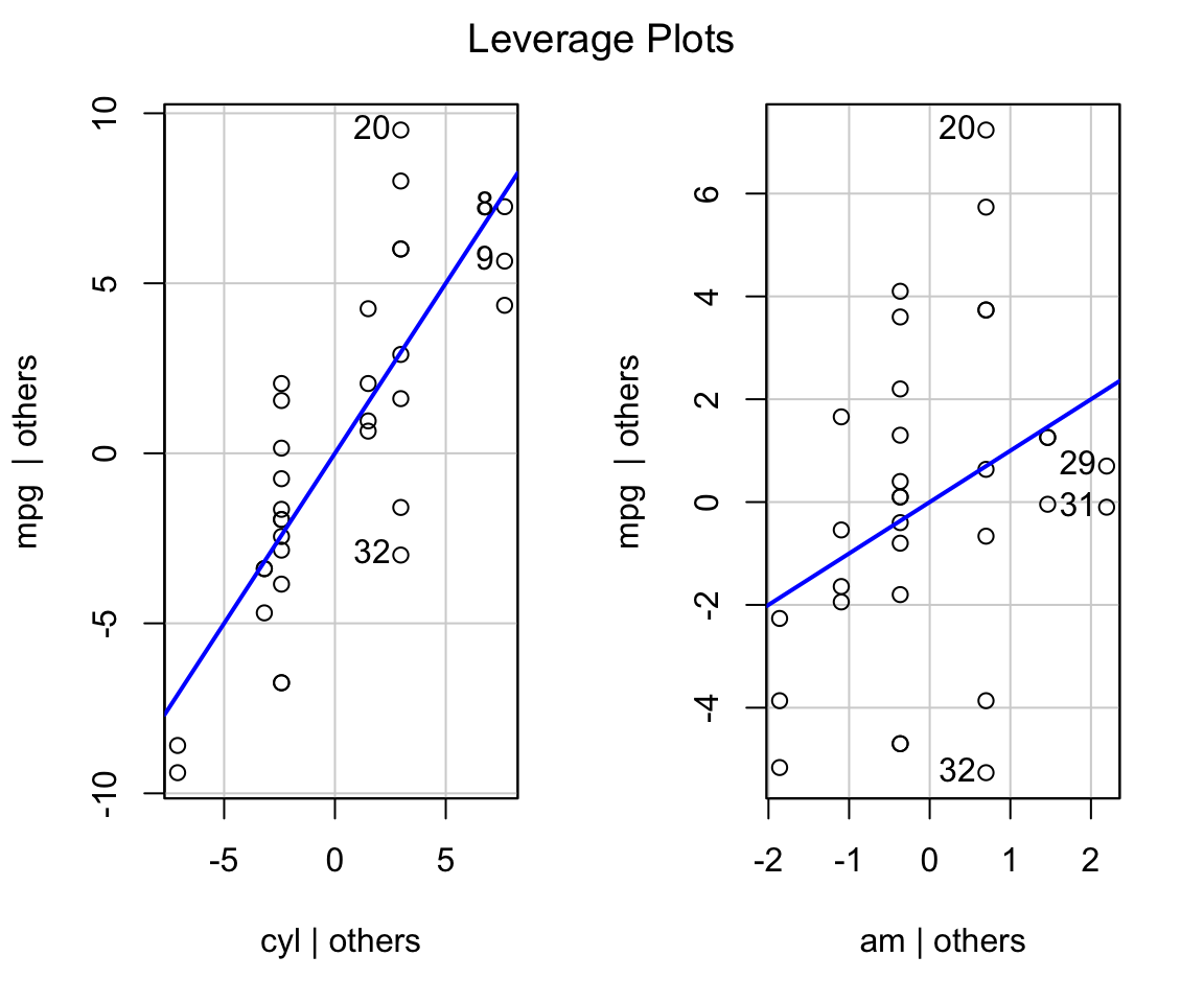
Relative Importance
# Relative Importance
library(relaimpo)
calc.relimp(stepBIC)
## Response variable: mpg
## Total response variance: 36.3241
## Analysis based on 32 observations
##
## 3 Regressors:
## Some regressors combined in groups:
## Group cyl : cyl6 cyl8
##
## Relative importance of 2 (groups of) regressors assessed:
## cyl am
##
## Proportion of variance explained by model: 76.51%
## Metrics are not normalized (rela=FALSE).
##
## Relative importance metrics:
##
## lmg
## cyl 0.5688862
## am 0.1962251
##
## Average coefficients for different model sizes:
##
## 1group 2groups
## cyl6 -6.920779 -6.156118
## cyl8 -11.563636 -10.067560
## am 7.244939 2.559954# See Predicted Value
pred = predict(stepBIC,dat3)
#See Actual vs. Predicted Value
finaldata = cbind(model, pred)
print(head(subset(finaldata, select = c(mpg, pred))))## mpg pred
## 1: 21.0 21.20569
## 2: 21.0 21.20569
## 3: 22.8 27.36181
## 4: 21.4 18.64573
## 5: 18.7 14.73429
## 6: 18.1 18.64573# As for the outlier that was identified above
print(subset(finaldata, select = c(mpg, pred))[20,])## mpg pred
## 1: 33.9 27.36181Manual Calculation of RMSE, Rsquared and Adjusted Rsquared
- For an in depth look at Box-Cox transformations see this site.
#Calculating RMSE
rmse <- sqrt(mean((dat3$mpg - pred)^2))
print(rmse)
## [1] 2.874977#Calculating Rsquared manually
y = as.list(dat3[,c("mpg")])
R.squared = 1 - sum((y$mpg - pred)^2)/sum((y$mpg - mean(y$mpg))^2)
print(R.squared)## [1] 0.7651114#Calculating Adj. Rsquared manually
n = dim(dat3)[1]
p = dim(summary(stepBIC)$coeff)[1] - 1
adj.r.squared = 1 - (1 - R.squared) * ((n - 1)/(n - p - 1))
print(adj.r.squared)## [1] 0.7399447#Box Cox Transformation
library(lmSupport)
modelBoxCox(stepBIC)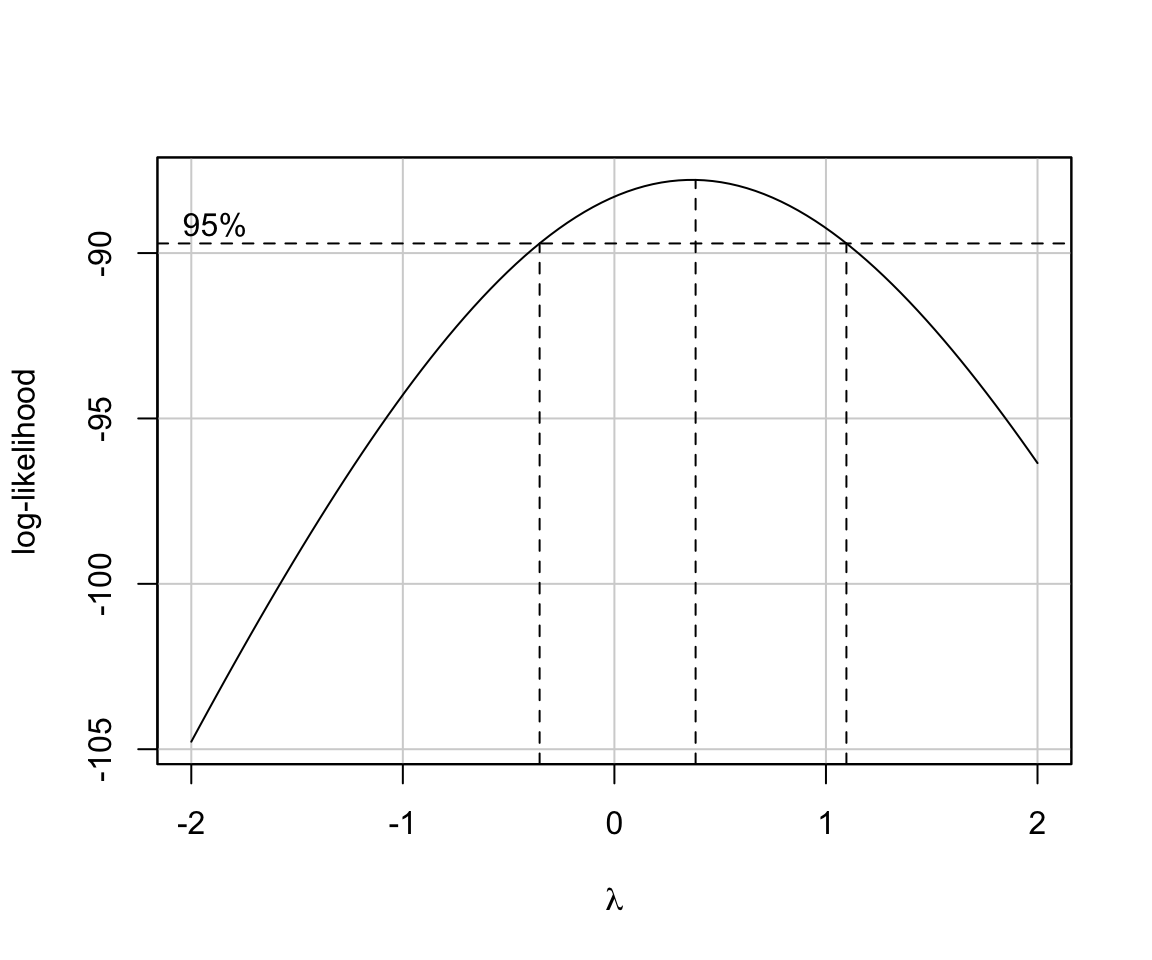
## [1] "Best Lambda= 0.38"
## [1] "Chi-square (df=1)= 3.01"
## [1] "p-value= 0.08285"
Summary
- Linear regression has been around for a long time, and is still very important for quantitative predictions. Frankly, this blog only scratches the surface on linear regression. At each step, there are many ways to conduct each analysis. Personally, I look forward to learning more and more ways to approach linear regression, as it is a foundational to many other tests that are more sophisticated. Until next time…