Logical Operators

• Both logical operators, such as and (&), or (|), and not equal to (!=), and arithmetic operators, such as addition (+) and multiplication (*) are used within the bracket to subset rows and columns.

# Use logical expressions with bracket notation to subset. In this example, all records that are greater than or equal to a Sepal.Width of 3.8, are subsetted.  See the 6 records that met the conditions below.
df <- iris[iris$Sepal.Width > 3.8,]
kable(df) %>%
  kable_styling(bootstrap_options = "striped", full_width = F)

• Another example.

# Use the '$' operator when subsetting with column names in the bracket.
df <- iris[iris$Petal.Length > 6 & iris$Sepal.Length < 7.3,]
kable(df) %>%
  kable_styling(bootstrap_options = "striped", full_width = F)

Data Aggregation

• To aggregate data, you have to use tapply, aggregate, and/or table. For example, get the mean of Sepal.Length:

# Use 'tapply' to find the mean Sepal.Length for each Species.  The 'tapply' function follows the format: (X, INDEX, FUN), where X is an atomic object, typically a vector, INDEX is a list of one or more factors, each of same length as X, and FUN is the function to be applied.  Since the data are already in a data.frame, the lengths are equal. The results show the mean 'Sepal.Length' for each 'Species'.
df <- tapply(iris$Sepal.Length, iris$Species, mean)
data.frame(df) %>%
mutate_if(is.numeric, format, digits=3, nsmall = 0) %>%
kable(.) %>%
  kable_styling(bootstrap_options = "striped", full_width = F)

# Examine the first 5 rows. Note there are three levels of 'Petal.Length', 1.3, 1.4, and 1.5.
df <- iris[1:5,]
kable(df) %>% 
  kable_styling(bootstrap_options = "striped", full_width = F)

# Use aggregate to find the mean of 'Sepal.Length' OF 'Species' GROUPED BY 'Petal.Length' (remeber, there are three levels). Highlight the 'aggregate' function in your RStudio editor and then hit F1 to open up the reference material for this function.
df <- aggregate(Sepal.Length[1:5] ~ Species[1:5] + Petal.Length[1:5], data = iris, mean)
kable(df) %>%
  kable_styling(bootstrap_options = "striped", full_width = F)

• Thus, for plants grouped by Petal.Lengths (1.3, 1.4. and 1.5), the calculated means (of Species within these groups, only “setosa” in this case) are equal to 4.7, 5.0, and 1.5. Note that the data is sorted on the GROUP BY in ascending order.

Subsetting Rows Using i

# or dt[3:5], Subset rows by number, similar to data.frame.
dt <- data.table(iris[3:5,])
kable(dt) %>% 
  kable_styling(bootstrap_options = "striped", full_width = F)  

# Subset on column names to select rows that satisfy the condition. dt[Species == "setosa"]. The [1:5] shows the first 5 rows, without this the whole data set is displayed (a feature not available with a data.frame)
dt <- dt[Species == "setosa",][1:5]
kable(dt) %>% 
  kable_styling(bootstrap_options = "striped", full_width = F) 

# Select on multiple values in a column.
dt <- dt[Species %in% c("setosa", "versicolor")][48:52]
kable(dt) %>% 
  kable_styling(bootstrap_options = "striped", full_width = F) 

Manipulate on Columns in j

# dt[,Species] returns a vector [1] "sestosa"....."versicolor", etc..
# Subset multiple columns with dot notation, which are returned as a data.table.  This is a very nice way to reduce the dimension of data you're interested in and work with smaller tables. Note that the .() is an alias of a list. If it is not used, the results returned are a vector.
dt <- dt[,.(Species, Sepal.Length)][48:52]
kable(dt) %>% 
  kable_styling(bootstrap_options = "striped", full_width = F)

Call functions in j.

dt <- data.table(iris)
dt <- c(dt[,length(Sepal.Length)], 
        dt[,sum(Sepal.Length)], 
        dt[,mean(Sepal.Length)], 
        dt[,sd(Sepal.Length)])
data.table(dt) %>%
mutate_if(is.numeric, format, digits=2, nsmall = 0) %>%
kable(.) %>% 
  kable_styling(bootstrap_options = "striped", full_width = F)

• How about all of these functions in one formula.

# use the combine functions to perform multiple functions on the same column
dt <- data.table(iris)
dt <- dt[,c(length(Sepal.Length), 
              sum(Sepal.Length), 
              mean(Sepal.Length), 
              sd(Sepal.Length))] 

# create a list of names
names(dt) <- c("Length", "Sum", "Mean", "Standard Deviation") 

# Return the vector of results with names for a report. Easy, and saves coding and lots of time.
data.table(dt) %>%
  mutate_if(is.numeric, format, digits=2, nsmall = 0) %>%
  kable(.) %>% 
  kable_styling(bootstrap_options = "striped", full_width = F)

• If the column lengths are different, the 2nd column will get recycled. Multiple expressions can also be wrapped into {} brackets in the j position. Such as {print(Species) plot(Sepal.Length) NULL}

# Use bracket notation similar to data.frame; the return carriage must be used to perform each wrapped function.
# dt[, {print(Species[1:5]) 
#       plot(Sepal.Length) 
#       NULL}] 

# Or use the dot notiation and commas to avoid the return carriage.  What ever you prefer. 
dt <- data.table(iris)
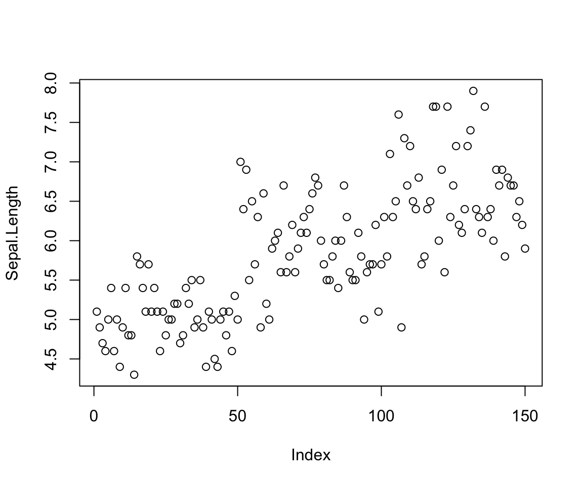
dt <- dt[,.(print(Species[1:5]), plot(Sepal.Length), NULL)]

[1] setosa setosa setosa setosa setosa Levels: setosa versicolor virginica

data.table(dt) %>%
  mutate_if(is.numeric, format, digits = 2, nsmall = 0) %>%
  kable(.) %>% 
  kable_styling(bootstrap_options = "striped", full_width = F)

Doing j BY Group

# use the dot notation to provide labels to the column.
dt <- data.table(iris)
dt <- dt[ ,.(Results = c(length(Sepal.Length), 
                           sum(Sepal.Length), 
                           mean(Sepal.Length), 
                           sd(Sepal.Length))), 
            by = "Species"] 

# create a list of names that are then applied to a column. Save time by using the length of the number of levels found from the by-selector.
dt$Category <- rep(c("Length", "Sum", 
                       "Mean", "Standard Deviation"),
                     length(levels(data$Species))) 

# Returns a data.table of results for a report. Easy, and saves time.
data.table(dt) %>%
  mutate_if(is.numeric, format, digits = 2, nsmall = 0) %>%
  kable(.) %>% 
  kable_styling(bootstrap_options = "striped", full_width = F)

# Group by several factors using the dot nottion .(X, Y).
dt <- data.table(iris)
dt <- dt[,.("Mean" = mean(Sepal.Length)), 
         by =.("Species" = Species, 
              "Petal Length" = Petal.Length)][1:5]
data.table(dt) %>%
  mutate_if(is.numeric, format, digits = 2, nsmall = 0) %>%
  kable(.) %>% 
  kable_styling(bootstrap_options = "striped", full_width = F)  

# Count the sum by multiple columns. This is a great feature!!  By the way, you can perform functions within the dot notation in the by bracket notation also.
dt <- data.table(iris)
dt <- dt[,.N,by = .(Species, Petal.Length)][1:5]
kable(dt) %>% 
  kable_styling(bootstrap_options = "striped", full_width = F)

Adding/Updating Columns By Referencing in j Using :=

# let's create a subset to work with first
dtt <- data.table(iris[1:5,])

kable(dtt) %>% 
  kable_styling(bootstrap_options = "striped", full_width = F)

• use the := to update a value in a column

# test$Sepal.Length  ......  [1] 5.1 4.9 4.7 4.6 5.0
dt <- dtt[, Sepal.Length := exp(Sepal.Length)]

# use the combine function to update multiple columns at the same time.
kable(dt) %>% 
  kable_styling(bootstrap_options = "striped", full_width = F)

• using functional :=

# test[,X := NULL] # removes a column instanly
# test[,c(X, Y) := NULL] # removes two columns
# Cols.chosen = c("Species", "Sepal.Width") # define columns
# test[, (Cols.chosen) := NULL] # removes columns based on the names in the vector
dt <- data.table(dtt[, ':=' (test = exp(Sepal.Length)),
                      by = Petal.Length][]) 
data.table(dt) %>%
  mutate_if(is.numeric, format, digits = 2, nsmall = 0) %>%
  kable(.) %>% 
  kable_styling(bootstrap_options = "striped", full_width = F) 

• Finally, there are many advanced features, indexing and key functions that enhance data.table operations. Several websites and blogs have shown that data.table operations much more efficient than data.frames.
• Although it will take some time to master the data.table, it will save you tons of time in the future, computationally and writing code. Until next time…